An axial flow pump curve plots head, efficiency, shaft power, and required suction head against flow rate at one stated speed, blade pitch, and impeller diameter. Read it by fixing a flow rate, tracing each curve at that flow rate, then finding where the head curve crosses your system curve. That crossing is the duty point, and the power curve tells you what the motor must survive there.
Most curve-reading mistakes start before the arithmetic. A buyer compares a headline efficiency number, or one duty point, with a pump selected at another speed or blade angle. The comparison looks tidy, but it mixes two configurations.
The method below reads the axial flow pump curve on one flow axis and one configuration. You will see how to read the four curves, test the duty point against seasonal system curves, and check what a catalog sheet cannot answer. The numbers are invented so you can follow the arithmetic without mistaking it for certified supplier data.
Key Takeaways
- An axial flow pump curve is a set of curves sharing one flow axis, not a single line.
- Axial pumps usually lose head quickly as flow rises, and some draw maximum power near shutoff.
- The duty point is where the pump head curve on the axial flow pump curve meets the system curve, not the midpoint of the published range.
- For the example in this article, 3,000 m³/h at 5 m needs about 40.9 kW of hydraulic power, 54.5 kW at the shaft, and 58.6 kW at the motor input.
- A single catalog row is one tested or listed condition, not a complete axial flow pump curve.
Those five statements explain why two buyers can read the same PDF and reach different conclusions. One reads the head line only, while the other reads the full axial flow pump curve, checks the power and suction curves at the same flow, and asks whether the installed system can hold that flow as water levels change. This guide follows the second approach.
Next step: If you already have a model in mind, compare its published condition with the submersible axial flow pump product page and request the curve at your actual speed and blade angle.
How to Read an Axial Flow Pump Curve
Start with the chart header, not the lines. A usable axial flow pump curve names the model, speed, blade angle, impeller diameter, liquid, and the test basis for the quoted flow rate. Without those settings, the curves describe a different machine or a different duty, so check them before you trace anything.
Then identify the axes. Flow rate belongs on the horizontal axis, and head belongs on the vertical axis. Every vertical read starts from one flow rate.
Some datasheets add efficiency, shaft power, and net positive suction head required (NPSHR) as separate panels, and others overlay them with separate vertical scales. Overlaid panels are harder to read, so fix one flow value and read each scale independently.
Follow this sequence at the flow you expect:
- Mark the flow on the horizontal axis.
- Move vertically to the head curve and record the head.
- Continue on the same vertical line to the efficiency curve and record the percentage.
- Read shaft power at that flow, not at the best efficiency point (BEP).
- Read NPSHR at the same flow and compare it with the net positive suction head available (NPSHa) on site.
- Repeat at the lowest flow rate and the highest flow rate your station will command.
The last step matters because an axial flow pump curve is steep. A small head change moves flow much further than it would on a low specific speed pump, so a station comfortable at design flow can run far to either side during a wet season.
The Four Curves on the Sheet
A complete axial flow pump curve usually contains four curves on one flow rate axis. The head curve shows the pressure energy added at each flow rate. The efficiency curve shows how much shaft power becomes hydraulic power.
The power curve shows shaft input, or sometimes motor input, depending on the supplier. The NPSHR curve shows the suction head needed to avoid unacceptable cavitation.
Read the legend before you compare numbers. A power curve labeled “input power” may mean power at the pump shaft, while a motor nameplate describes electrical input. A curve labeled “water horsepower” describes hydraulic output, as one manufacturer notes on its axial flow curve downloads.
Those are three different quantities. Mixing them is one of the most common reading errors.
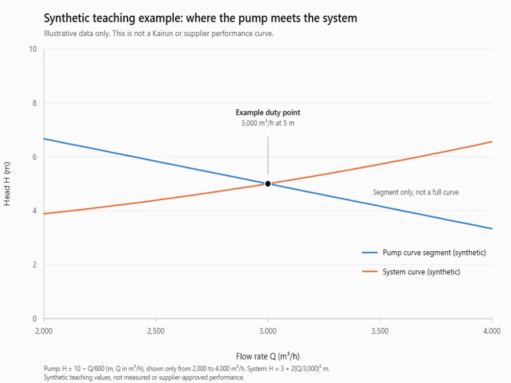
Figure 1. A synthetic axial flow pump curve segment and a synthetic system curve. The values are teaching inputs, not a Kairun or supplier performance curve.
| Flow (m³/h) | Pump head (m) | System head (m) |
|---|---|---|
| 2,400 | 6.00 | 4.28 |
| 3,000 | 5.00 | 5.00 |
| 3,600 | 4.00 | 5.88 |
The pump line uses a teaching relation, H = 10 − Q/600, plotted only from 2,000 to 4,000 m³/h. It stops short of shutoff, where a real axial flow pump curve can turn or become unstable. The system line uses H = 3 + 2(Q/3,000)² m. Both are invented, and neither proves how any Kairun model behaves.
What Makes an Axial Flow Pump Curve Different?
Specific speed explains most of the shape of the axial flow pump curve. Axial flow machines move large volumes at low head, and their head curve falls steeply as flow rises. KSB’s characteristic curve reference shows an axial flow example and notes two consequences of high specific speed: a steeper head curve and a sharper efficiency peak. It also states that power input peaks at zero flow for that type.
That power behavior changes how you protect the motor. On many low specific speed centrifugal pumps, power falls as flow falls. On an axial flow pump, throttling toward a low flow rate can raise the absorbed power. A startup, a closed valve, or a control sequence that chases a low flow setpoint can therefore overload a motor that looked adequate at the design duty point.
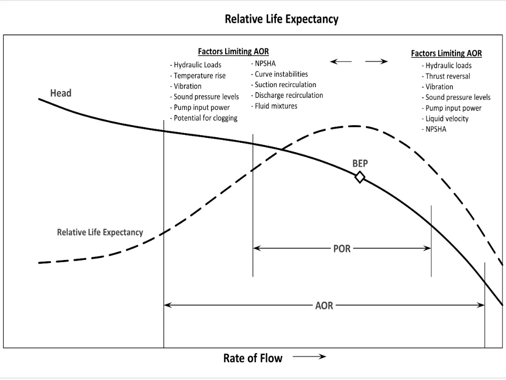
Low flow also raises mechanical and hydraulic risk. The Hydraulic Institute’s pump curve tutorial explains BEP, the preferred operating region (POR), and the allowable operating region (AOR). The AOR is set by the manufacturer and can be limited by cavitation, heating, vibration, noise, shaft deflection, or fatigue. A published head curve alone does not define it.
Read the Efficiency Peak, Then the Limits
The BEP is the flow rate where efficiency is highest at a given speed and impeller diameter, and efficiency falls on both sides of that peak. The farther the duty point sits from BEP on the axial flow pump curve, the more energy the station spends for the same water moved, and the more hydraulic load the pump carries.
Do not assume the same percentage band applies to every axial pump. The Hydraulic Institute notes that the POR can range from about 70 to 120 percent of BEP flow for some pumps and from about 90 to 110 percent for others, depending on specific speed. For axial and mixed flow machines, the manufacturer must define the actual AOR. Ask for that boundary in writing, including minimum flow and any unstable region.
Fictional scenario: Mara, a project engineer for a drainage station, compared two bids by their BEP efficiency. Model A looked better by two points. When she overlaid each quoted curve with the station’s seasonal system curves, Model A spent most of the flood season at 55 percent of BEP flow, inside a region the supplier had excluded from its AOR.
Model B had a lower peak efficiency but held the duty point inside its AOR at both low and high water levels. That comparison changed the recommendation, even though the headline efficiency numbers did not.
Find the Intersection With the System Curve
An axial flow pump curve describes the machine, and a system curve describes the plant. The pump will operate where the two intersect, because that is the only flow rate where the head the pump produces equals the head the system demands.
The Hydraulic Institute’s system curve guide splits system head into static head and frictional head. Static head comes from elevation and pressure differences between the source and destination. Friction comes from pipe length, fittings, valves, and changes in direction, and it rises roughly with the square of flow when the system geometry stays fixed.
For a flood-control station, static head is not one number. It changes with river level, wet-well level, and discharge level. Draw one system curve for low water, a second system curve for normal operation, and a third system curve for the flood case.
Mark where each crosses the axial flow pump curve. One duty point is not enough evidence for a station that must work across a season.
Work Through One Duty Point
On this teaching axial flow pump curve, use the synthetic example in the figure. At 3,000 m³/h, the pump head is 5 m. The system curve also needs 5 m at that flow rate, so 3,000 m³/h is the example duty point.
At 2,400 m³/h the pump offers 6 m while the system curve needs 4.28 m, so flow rises. At 3,600 m³/h the pump offers 4 m while the system curve needs 5.88 m, so flow falls. The intersection is stable.
Now size the power. Hydraulic power is:
P_h = ρ × g × Q × H / 1,000
With water at about 1,000 kg/m³, gravity at 9.81 m/s², Q = 3,000 m³/h (0.8333 m³/s), and H = 5 m, the hydraulic power is about 40.9 kW. If the pump efficiency at that flow rate is 75 percent, shaft power is 40.9 / 0.75 = 54.5 kW. If the motor efficiency is 93 percent, motor input is about 58.6 kW before variable frequency drive and cable losses. Those are illustrative assumptions, not a motor selection.
This is where a simple axial flow pump curve reading becomes a purchasing decision. A 55 kW motor leaves almost no margin at the assumed shaft power. A 75 kW motor may be safer, but the answer depends on the actual curve, service factor, ambient conditions, and starting method. Do not let a catalog table’s power column decide that alone.
Fictional scenario: Daniel, an EPC mechanical lead, sized a station motor from the power value printed beside a pump’s rated flow. The value looked like absorbed power. During commissioning, the pump ran at a lower flow while the discharge level rose, and the motor current climbed above the nameplate value.
The supplier then confirmed that the printed number was a recommended motor rating, not the power at that exact flow. Daniel replaced the motor protection settings and added a minimum-flow interlock, but the station lost two weeks. The table had not lied. It had simply answered a narrower question than the one he asked.
Next step: Before you fix a motor size, send the pump supplier your three system curves and ask for shaft power at each intersection. Our engineers can review the duty with you through the contact page.
Check Speed, Blade Pitch, and Parallel Operation
Speed changes the axial flow pump curve. With fixed geometry, the affinity rules say flow rate varies with speed, head with speed squared, and power with speed cubed. They assume the same efficiency and apply within the limits of the relevant standard. They are not a license to rescale the curve across the full range.
Take the synthetic duty point at 3,000 m³/h and 5 m. Reduce speed by 10 percent. The homologous point becomes 2,700 m³/h at 4.05 m.
A reader might stop there and announce a new duty point. That would be wrong.
At 2,700 m³/h the same system needs about 4.62 m, so the system curve no longer passes through the mapped point. The real intersection, and the new duty point, is elsewhere, near 2,485 m³/h at 4.37 m in this synthetic case. Redraw the pump curve and solve again.
Blade pitch works differently. An axial pump curve is normally published at a stated blade angle. Changing pitch changes the head-flow relation and the power demand, but the shift depends on the hydraulic design and the adjustment range.
Do not take a curve at one pitch and assume the same efficiency or the same low-flow limit at another. Ask for a curve family at the pitches you will actually use, with the safe adjustment envelope marked.
Parallel operation adds another layer. At any common head, add the flow rates of the running pumps to build a combined curve. The combined curve crosses the system curve at a higher flow, but the increase is rarely double.
The Hydraulic Institute notes that a second pump does not double flow unless the system curve is almost flat. Suction intake conditions can also limit what the added pump can deliver.
Next step: If flow varies across the season, compare fixed-speed and variable-speed options on the same system curves. Our submersible pump VFD guide covers the site checks that belong beside that comparison.
Check Suction Conditions Before Accepting the Duty Point
NPSHR is part of the axial flow pump curve, and it rises with flow rate on most published sheets. NPSHa comes from the site: atmospheric pressure, the water surface above the impeller, and the vapor pressure of the liquid. The pump needs NPSHa above NPSHR with a margin that suits the application, the measurement uncertainty, and the operating range. A curve point without a suction check at the duty point is incomplete.
Submergence is a separate question, and the Hydraulic Institute’s submergence guidance defines it as the depth from the free surface to the pump inlet, and ties minimum submergence to vortex prevention as well as NPSH. A pump can meet its NPSHR and still pull air because the intake is too shallow, the approach flow is uneven, or the sump geometry creates a vortex. Those are intake design issues, not curve corrections.
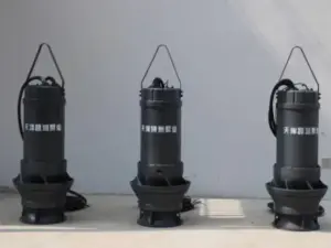
For a submersible axial flow pump, the motor is in the same water as the impeller, and that does not remove the need for suction-side checks. Confirm the minimum submergence for your intake, the clearance to the floor, and the approach conditions with the supplier. Suction conditions can move the usable duty point even when the head curve looks acceptable. If cavitation risk is already showing in operation, our guide to pump cavitation causes and prevention explains the field symptoms.
Questions About the Axial Flow Pump Curve
Is there one axial flow pump curve PDF for every model? No. Each curve belongs to a model, speed, blade angle, impeller diameter, and test basis. A generic PDF cannot define the performance of a different configuration. Use a model-specific axial flow pump curve for selection.
Why does power rise at low flow on some axial pumps? High specific speed changes the shape of the power curve. KSB notes that power input reaches a maximum at zero flow for its axial flow example. Confirm the behavior on your model’s axial flow pump curve and set the minimum flow and motor protection accordingly.
Does a second pump double the flow? Usually not. Add the pump flow rates at the same head, then read the new intersection with the system curve. Friction and static head decide how much it adds. Plot the combined curve against each system curve.
Can I use the catalog table as the axial flow pump curve? Only as a starting point.
A table row is one listed condition, not a system curve. The Kairun QZ table, for example, lists 350QZ-100D at 0° vane angle, 802.9 m³/h, 1.92 m, 11 kW, 1,450 r/min, 79.5 percent efficiency, and a 300 mm impeller. That row does not define the full axial flow pump curve, the AOR, or the NPSHR at other flows. Ask which quantity the power column represents before you compare it with a motor rating.
Turn the Curve Into a Selection Decision
An axial flow pump curve is a map of possibilities, not a promise for your station. The useful duty point appears only after you overlay your system curves, check the power and NPSHR at the same flow, and confirm the operating range with the manufacturer. Do that work before the order, not after commissioning.
For your next inquiry, send five items: design flow rate and head range, the lowest and highest system curves, allowable blade pitch or speed range, suction and submergence conditions, and the power definition on the curve. Ask for the model-specific axial flow pump curve at the proposed setting, with the AOR and NPSHR included. Then compare the intersection on each system curve, not the headline efficiency alone.
Your next step
If you have the flow rate, head, and site conditions, our engineers can review the duty and identify the curve data you still need. Tell us your application through the Kairun contact page and ask for a model-specific curve before you commit to a motor or a station design. A clear curve review now is cheaper than a motor replacement later.