Axial flow pump power consumption depends on flow rate, total head, and the efficiencies of the pump, motor, and drive. Calculate hydraulic output first, then add the effect of losses to find electrical input power. Multiply that kW by running hours to estimate kWh.
Here’s the surprise: restricting an axial flow pump can raise its load. A smaller flow reading doesn’t always mean a smaller electricity bill. That makes a nameplate-only estimate a poor basis for your energy cost budget. Seasonal changes in water level add to the problem.
You need a calculation you can check. Every power boundary needs a clear name. This guide connects flow and head to pump efficiency, electrical demand, annual energy, and field measurements. It also explains why a variable frequency drive (VFD) needs a system-curve check before anyone promises savings.
The worked examples use assumed teaching inputs, not Kairun test results or customer records. Use them to organize your own site data.
Then check axial flow pump power consumption against the exact pump curve and suitable power readings. The goal is a sound estimate for your water duty.
Key Takeaways
- Hydraulic output, shaft input, and electrical input are different kW values; pump efficiency alone doesn’t describe the whole electrical chain.
- Axial flow pump power consumption can rise at low flow, so check the manufacturer’s power curve and permitted operating range.
- Annual electricity equals the sum of each operating period’s electrical kW multiplied by its hours.
- At corresponding points, 80% speed suggests 51.2% shaft power under similarity assumptions; actual station savings require a separate assessment.
Next step: Have flow and head figures but no clear power boundary? Discuss your duty point with Kairun Pump and include the curve or power data you’re comparing.
How to Calculate Axial Flow Pump Power Consumption
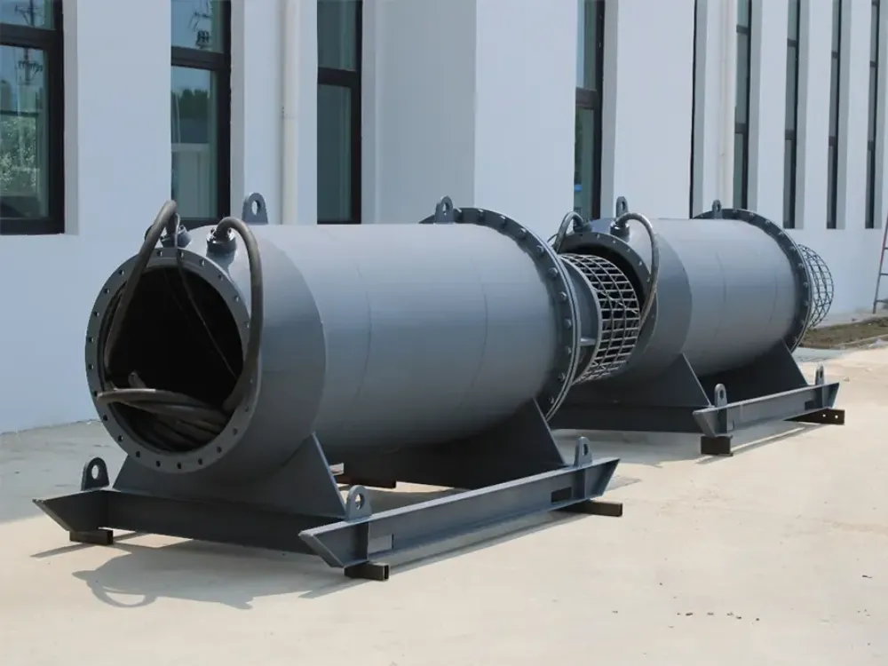
Separate hydraulic, shaft, and electrical power
Start an axial flow pump power consumption estimate with flow rate Q and total dynamic head H. Head is the energy added per unit weight of liquid, expressed in meters. Across a system, it includes lift, pressure difference, and losses that change with flow. A single discharge-pressure reading may not describe it.
For liquid density ρ in kg/m³ and Q in m³/s:
Hydraulic power [kW] = ρ × 9.81 × Q × H / 1,000
If Q is in m³/h, divide by 3,600,000 instead. Then divide hydraulic output by pump efficiency to find shaft input power. For a direct-driven pump with a VFD, divide again by motor and drive efficiencies. This gives an estimate at the drive’s line-side input.
The DOE pumping system sourcebook sets out fluid power, shaft power, and electrical input as distinct values. Its measurement and cost guidance also explains why operating demand matters more than a motor label.
Follow one worked example through every boundary
Fictional scenario: Lina, an irrigation project engineer, needs a first budget for 3,000 m³/h at 5 m total head. They assume clean water at 1,000 kg/m³, pump efficiency of 75%, motor efficiency of 93%, and drive efficiency of 97%. The results below let Lina trace each loss. These are teaching values.
| Power boundary | Calculation with assumed inputs | Result |
|---|---|---|
| Hydraulic output | 1,000 × 9.81 × (3,000 / 3,600) × 5 / 1,000 | 40.875 kW |
| Pump shaft input | 40.875 / 0.75 | 54.5 kW |
| Motor electrical input | 54.5 / 0.93 | 58.60 kW |
| Drive line input | 58.60215 / 0.97 | 60.41 kW |
Lina uses 60.4 kW as a rounded budgeting figure. At 2,000 hours, that gives 120,800 kWh. An assumed USD 0.12/kWh gives an energy cost of USD 14,496. Using unrounded power instead gives about 120,829 kWh and USD 14,499.50; use one rounding method throughout.
This axial flow pump power consumption calculation leaves out other station loads and extra cable or transmission losses. Include them when your boundary requires it. Also, pump efficiency must come from the duty point in question. A peak catalog value won’t cover every water level.
Before comparing axial flow pump options, ask whether each curve’s power axis means shaft or electrical input. Motor rated kW normally states its rated mechanical output. It isn’t a reading of electrical input power in service. A valid energy cost comparison starts with matching those definitions.
Why Axial Flow Pump Power Consumption Rises at Low Flow
Read the curve before restricting discharge
Axial flow pump power consumption can behave differently from the radial pump curve you remember. KSB’s characteristic curve reference describes high-specific-speed pumps whose input power reaches a maximum at shutoff. That is a trend in the curves. It doesn’t give one kW value for every design.
At zero delivered flow, useful hydraulic output approaches zero. The impeller can still draw high shaft input power.
Losses and fluid motion within the pump account for that load. Don’t hold pump efficiency constant at shutoff. The normal-duty formula can’t then prove that the pump needs no power.
When investigating axial flow pump power consumption, use the curve for the exact model, speed, and blade setting. Check its allowed range and the motor loading across that range. One good duty point doesn’t prove that every other point is safe. A low flow reading doesn’t prove low load either.
Understand separation and recirculation
At low flow, liquid can meet the blades at a poor angle. Flow can then break away from their surfaces.
Flow can also turn back within the pump, called recirculation. Pump efficiency can fall, and vibration can rise. KSB’s operating behaviour guidance explains these mechanisms and the operating limits of high-specific-speed pumps.
These effects help explain unexpected axial flow pump power consumption. A bill alone, though, can’t show which fault is present.
Log flow, head, speed, vibration, and input power together. Before changing controls, check the readings against the maker’s limits. These include limits for continuous and brief runs.
Don’t use throttling or a closed-valve run as a generic energy-saving test. Follow the exact equipment’s startup and operating procedures. There isn’t one minimum flow or VFD frequency that fits all sites.
Turn Electrical kW Into Annual kWh and Cost

Build a duty-and-hours table
Axial flow pump power consumption in kW is a rate at a given moment. Energy in kWh also depends on how long each condition lasts. For changing duty, use Annual kWh = Σ(electrical kW × hours). The sum covers each duty period, not one reading stretched across a year.
Fictional scenario: Omar manages a drainage station’s planning spreadsheet. They assume two operating periods: 65 kW for 2,000 hours and 40 kW for 1,000 hours. The total is 170,000 kWh, with an energy cost of USD 20,400 at an assumed USD 0.12/kWh. Omar now has a budget by duty period; these aren’t customer records.
| Assumed operating period | Electrical input power | Hours per year | Energy |
|---|---|---|---|
| Higher-demand period | 65 kW | 2,000 | 130,000 kWh |
| Lower-demand period | 40 kW | 1,000 | 40,000 kWh |
| Total | Varies with duty | 3,000 | 170,000 kWh |
For a real axial flow pump power consumption budget, add flow, head, and water levels to each row. Note how many pumps are running too.
Pump efficiency and motor loading may change between periods. A lower yearly total may just mean less water moved. It doesn’t prove better performance.
Keep energy charges separate from the full bill
Calculate energy cost using the tariff that applies to each period. Time-of-use prices can change the result even if annual kWh stays constant. Your tariff may also include demand charges, fixed fees, taxes, or power-factor penalties. Work these out on their own.
To compare axial flow pump power consumption per delivered volume, divide metered kWh by cubic meters delivered. Compare the same lift and service.
A higher lift calls for more useful hydraulic work. Count other station loads on the same basis. Otherwise, the energy cost gap may come from different meter boundaries.
Next step: Prepare your operating-period table and send your operating data. Include flow, head, annual hours, tariff assumptions, and the location of the power meter.
When VFD Speed Reduction Can Save Energy
Use the cube law at corresponding points
A VFD changes speed, which can help match pumping to demand. For axial flow pump power consumption, however, a speed ratio alone is only a screening input. The affinity laws compare corresponding points: matched points on curves at different speeds. They assume the same geometry and liquid, with roughly unchanged pump efficiency.
Call the speed ratio r. At corresponding points, flow ratio is r, head ratio is r², and shaft-power ratio is about r³.
These relationships describe the pump, not the complete electrical bill. Motor and drive losses also change. Electrical input power needs its own check.
At 80% speed, the relationships give 80% flow, 64% head, and 51.2% shaft power. That arithmetic doesn’t establish a 48.8% reduction in annual energy cost. You may need to run longer to deliver the same volume. Lower kW needn’t mean lower annual kWh.
Recheck static lift and operating limits
Static head is the lift or pressure difference that remains as friction losses fall. It can make up much of the required head.
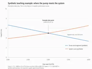
The lower-speed pump curve may then meet the system curve at a different relative flow. Pump efficiency can change. The reduced-speed curve may even fail to give a useful operating point.
This is why a speed setting alone can’t predict axial flow pump power consumption.
Fictional scenario: Mei reviews a flood-control concept at 80% speed. Their worksheet shows the 51.2% shaft-power ratio; a high receiving-water level changes the required lift. Mei leaves axial flow pump power consumption and annual energy cost open until the new duty point is found. They must check pump efficiency and hours too; the ratio is a screening step, not a promised saving.
Use the DOE sourcebook’s variable-speed material alongside the actual curves. For a site review, the submersible pump VFD checks cover related drive and motor considerations. Check motor cooling and how deep the pump must sit below water, called submergence. Confirm cable needs and allowed speeds for the actual equipment.
Compare speed control with pump staging, which changes the number of running pumps. Use only arrangements approved for the equipment. The best choice for axial flow pump power consumption depends on the required flow schedule and water-level range. Base the energy cost calculation on that same required service for each option.
Measure Axial Flow Pump Power Consumption at the Right Boundary

Log true power with flow and head
Measure axial flow pump power consumption with a suitable power meter. It must suit the supply and waveform at the chosen point. Line-side real kW includes drive losses.
A suitable drive-output reading has a different boundary. A station feeder may include other equipment. Label every meter location.
Don’t treat current in amperes, apparent power in kVA, or motor nameplate kW as measured real input power. Voltage and power factor matter too. Drive waveforms add further metering needs. Ordinary current readings or displacement power factor alone won’t establish true demand with a VFD.
Have qualified personnel arrange electrical measurements under the site’s procedures. Collect these readings over the same interval:
- True input power in kW and accumulated energy in kWh at the stated boundary
- Flow rate and the volume delivered during the interval
- Suction and discharge conditions needed to calculate total pump head
- Water levels, speed, blade setting where applicable, and number of operating pumps
- Relevant alarms, vibration observations, and any changes to valves or controls
Compare equivalent service before claiming savings
For a field check of axial flow pump power consumption, match the readings in time. The electrical and hydraulic data must describe the same duty. Divide hydraulic kW by line-side electrical kW to get wire-to-water efficiency.
This describes that whole boundary. Pump efficiency alone uses shaft input power. Label the distinction in your report.
Repeat readings across the main site conditions. Don’t treat a brief reading as the annual average.
Changing water levels or fouled passages can alter the duty point. The submersible pump maintenance checklist helps with related checks. A change in kW alone doesn’t prove wear.
To assess energy cost improvements, compare equal service with the same meter boundaries. State the likely error in the readings.
Record instrument suitability and any estimated hours. Someone else can then repeat your axial flow pump power consumption comparison. Lower input power alone doesn’t prove higher efficiency.
Frequently Asked Questions
How do I calculate an axial flow pump’s electrical power?
Calculate hydraulic kW as ρ × 9.81 × Q × H / 1,000, using Q in m³/s. Divide by the duty-point pump efficiency, motor efficiency, and drive efficiency where applicable. This estimates axial flow pump power consumption at the drive input. Add other losses or station loads if your boundary includes them.
Why can an axial flow pump draw more power at low flow?
Low-flow separation and recirculation can raise losses and shaft demand while pump efficiency falls. The exact behavior depends on the design, speed, and blade setting. Check the manufacturer’s power curve and allowed range. Don’t infer input power from flow alone or test by closing a valve.
Does a 20% speed reduction cut electricity use by 48.8%?
It doesn’t establish that electrical saving. The 0.8³ result is a 51.2% shaft-power ratio at corresponding points under affinity-law assumptions. Actual axial flow pump power consumption also depends on the system intersection, changing efficiencies, and losses. Annual energy cost depends on runtime and the tariff too.
Can motor nameplate kW or current tell me the running cost?
Neither value alone establishes running energy cost. Motor rated kW normally describes rated mechanical output.
Current lacks the full information needed for true electrical power. Measure real kW or kWh with suitable equipment at a defined boundary. Apply the hours and electricity prices that fit your site.
How should I compare two pumps’ annual energy costs?
Calculate each option’s electrical demand over the same flow, head, and operating-hours schedule. Use duty-point pump efficiency and the relevant motor and drive losses. Compare axial flow pump power consumption for the same delivered service. Use the same tariffs and other-load boundaries for both options.
Conclusion: Confirm the Duty Before Comparing Energy
Start with the water duty, then follow the power through each component. Flow and total head define useful hydraulic output. Pump efficiency connects that output to shaft demand. Motor and drive losses determine the next electrical boundary, while annual hours turn electrical kW into energy.
Check the actual power curve before changing how the pump runs. Low flow can mean higher demand. A lower-speed estimate needs a fresh system-curve check when static lift matters. Neither a catalog peak efficiency nor a single meter reading can represent every seasonal condition at your station.
Build a short, traceable worksheet with assumptions, duty periods, measurement points, and tariffs. Keep calculated values separate from observed readings, and compare the same delivered service. This makes an energy cost estimate easier to update as water levels or schedules change.
Next step: Send Kairun Pump your project inputs, including flow, total head, water-level range, hours, supply details, and available curves or measurements. Those inputs provide the basis for checking axial flow pump power consumption against your actual application.